A Appendix
This Appendix contains supplemental information about various aspects of R and ggplot that you are likely to run into as you use it. You are at the beginning of a process of discovering practical problems that are an inevitable part of using software. This is often frustrating. But feeling stumped is a standard experience for everyone who writes code. Each time you figure out the solution to your problem, you acquire more and more knowledge about how and why things go wrong, and more confidence about how to tackle the next glitch that comes along.
A.1 A little more about R
A.1.1 How to read an R help page
Functions, datasets, and other built-in objects in R are documented in its help system. You can search or browse this documentation via the “Help” tab in RStudio’s lower right-hand window. The quality of R’s help pages varies somewhat. They tend to be on the terse side. However, they all have essentially the same structure and it is useful to know how to read them. Figure A.1 provides an overview of what to look for. Remember, functions take inputs, perform actions, and return outputs. Something goes in, it gets worked on, and then something comes out. That means you want to know what the function requires, what it does, and what it returns. What it requires is shown in the Usage and Arguments sections of the help page. The names of all the required and optional arguments are given by name and in the order the function expects them. Some arguments have default values. In the case of the mean() function the argument na.rm is set to FALSE by default. These will be shown in the Usage section. If a named argument has no default, you will have to give it a value. Depending on what the argument is, this might be a logical value, a number, a dataset, or any other object.
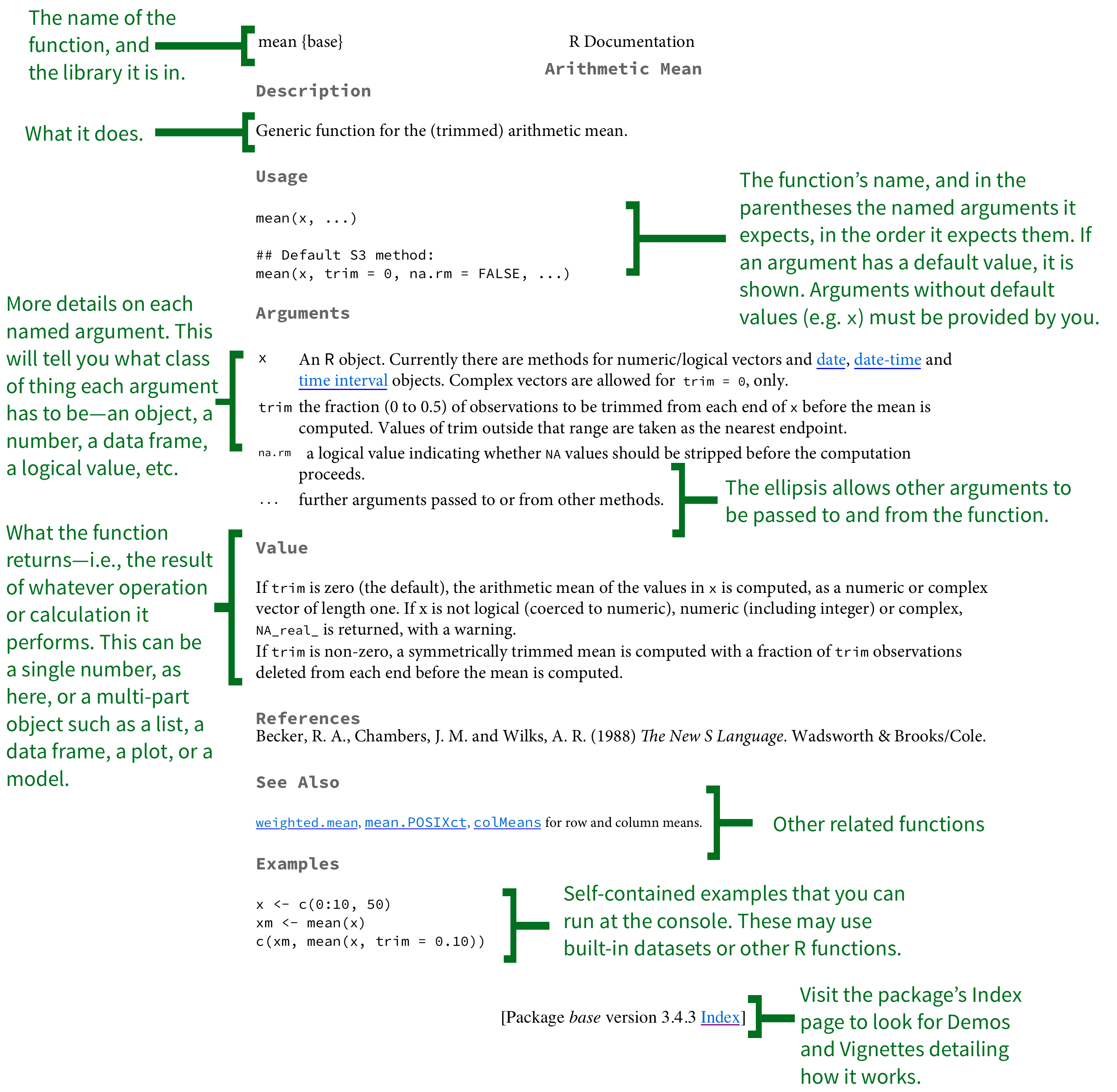
Figure A.1: The structure of an R help page.
The other part to look at closely is the Value section, which tells you what the function returns once it has done its calculation. Again, depending on what the function is, this might simply be a single number or other short bit of output. But it could also be something as complex as a ggplot figure or a model object consisting of many separate parts organized as a list.
Well-documented packages will often have Demos and Vignettes attached to them. These are meant to describe the package as a whole, rather than specific functions. A good package vignette will often have one or more fully-worked examples together with a discussion describing how the package works and what it can do. To see if there any package vignettes, click the link at the bottom of the function’s help page to be taken to the package index. Any available demos, vignettes, or other general help will be listed at the top.
A.1.2 The basics of accessing and selecting things
Generally speaking, the tidyverse’s preferred methods for data
subsetting, filtering, slicing and selecting will keep you away from
the underlying mechanics of selecting and extracting elements of
vectors, matrices, or tables of data. Carrying out these operations
through functions like select(), filter(), subset(), and
merge() is generally safer and more reliable than accessing elements
directly. However, it is worth knowing the basics of these operations.
Sometimes accessing elements directly is the most convenient thing to
do. More importantly, we may use these techniques in small ways in our
code with some regularity. Here we very briefly introduce some of R’s
selection operators for vectors, arrays, and tables.
Consider the my_numbers and your_numbers vectors again.
my_numbers <- c(1, 2, 3, 1, 3, 5, 25)
your_numbers <- c(5, 31, 71, 1, 3, 21, 6)
To access any particular element in my_numbers, we use square
brackets. Square brackets are not like the parentheses after
functions. They are used to pick out an element indexed by its
position:
my_numbers[4]## [1] 1my_numbers[7]## [1] 25Putting the number n inside the brackets will give us (or “return”) the nth element in the vector, assuming there is one. To access a sequence of elements within a vector we can do this:
my_numbers[2:4]## [1] 2 3 1This shorthand notation tells R to count from the 2nd to the 4th
element, inclusive. We are not restricted to selecting contiguous
elements, either. We can make use of our c() function again:
my_numbers[c(2, 4)]## [1] 2 1R evaluates the expression c(2,4) first, and then extracts just the
second and the fourth element from my_numbers, ignoring the others.
You might wonder why we didn’t just write my_numbers[2,3] directly.
The answer is that this notation is used for objects arrayed in two
dimensions (i.e. something with rows and columns), like matrices, data
frames, or tibbles. We can make a two-dimensional object by creating
two different vectors with the c() function and using the tibble()
function to collect them together:
my_tb <- tibble(
    mine = c(1,4,5, 8:11),
    yours = c(3,20,16, 34:31))

class(my_tb)
## [1] "tbl_df" "tbl" "data.frame"my_tb## # A tibble: 7 x 2
## mine yours
## <dbl> <dbl>
## 1 1.00 3.00
## 2 4.00 20.0
## 3 5.00 16.0
## 4 8.00 34.0
## 5 9.00 33.0
## 6 10.0 32.0
## 7 11.0 31.0WeIn these chunks of code you will see some explanatory text set off by the hash symbol, #. In R’s syntax, the hash symbol is used to designate a comment. On any line of code, text that appears after a # symbol will be ignored by R’s interpreter. It won’t be evaluated and it won’t trigger a syntax error. index data frames, tibbles, and other arrays by row first, and then by column. Arrays may also have more than two dimensions.
my_tb[3,1] # Row 3 Col 1## # A tibble: 1 x 1
## mine
## <dbl>
## 1 5.00my_tb[1,2] # Row 1, Col 2 ## # A tibble: 1 x 1
## yours
## <dbl>
## 1 3.00The columns in our tibble have names. We can select elements using them, too. We do this by putting the name of the column in quotes where we previously put the index number of the column:
my_tb[3,"mine"] # Row 3 Col 1## # A tibble: 1 x 1
## mine
## <dbl>
## 1 5.00my_tb[1,"yours"] # Row 1, Col 2 ## # A tibble: 1 x 1
## yours
## <dbl>
## 1 3.00my_tb[3,"mine"] # Row 3 Col 1## # A tibble: 1 x 1
## mine
## <dbl>
## 1 5.00my_tb[1,"yours"] # Row 1, Col 2 ## # A tibble: 1 x 1
## yours
## <dbl>
## 1 3.00If we want to get all the elements of a particular column, we can leave out the row index. This will mean all the rows will be included for whichever column we select.
my_tb[,"mine"] # All rows, Col 1## # A tibble: 7 x 1
## mine
## <dbl>
## 1 1.00
## 2 4.00
## 3 5.00
## 4 8.00
## 5 9.00
## 6 10.0
## 7 11.0We can do this the other way around, too, selecting a particular row and showing all columns:
my_tb[4,] # Row 4, all cols## # A tibble: 1 x 2
## mine yours
## <dbl> <dbl>
## 1 8.00 34.0A better way of accessing particular columns in a data frame is via
the $ operator, which can be used to extract components of various
sorts of object. This way we append the name of the column we want to
the name of the object it belongs to:
my_tb$mine## [1] 1 4 5 8 9 10 11Elements of many other objects can be extracted in this way, too, including nested objects.
out <- lm(mine ~ yours, data = my_tb)

out$coefficients
## (Intercept) yours
## -0.0801192 0.2873422out$call## lm(formula = mine ~ yours, data = my_tb)out$qr$rank # nested ## [1] 2Finally, in the case of data frames the $ operator also lets us add new columns to the object. For example, we can add the first two columns together, row by row. To create a column in this way, we put the $ and the name of the new column on the left-hand side of the assignment.
my_tb$ours <- my_tb$mine + my_tb$yours
my_tb
## # A tibble: 7 x 3
## mine yours ours
## <dbl> <dbl> <dbl>
## 1 1.00 3.00 4.00
## 2 4.00 20.0 24.0
## 3 5.00 16.0 21.0
## 4 8.00 34.0 42.0
## 5 9.00 33.0 42.0
## 6 10.0 32.0 42.0
## 7 11.0 31.0 42.0In this book we do not generally access data via [ or $. It is
particularly bad practice to access elements by their index number
only, as opposed to using names. In both cases, and especially the
latter, it is too easy to make a mistake and choose the wrong columns
or rows. In addition, if our table changes shape later on (e.g. due to
the addition of new original data) then any absolute reference to the
position of columns (rather than to their names) is very likely to
break. Still, we do use the c() function for small tasks quite
regularly, so it’s worth understanding how it can be used to pick out
elements from vectors.
A.1.3 Tidy data
Working with R and ggplot is much easier if the data you use is in the right shape. Ggplot wants your data to be tidy. For a more thorough introduction to the idea of tidy data, see Chapters 5 and 12 of Wickham & Grolemund (2016). To get a sense of what a tidy dataset looks like in R, we will follow the discussion in Wickham (2014). In a tidy dataset,
- Each variable is a column.
- Each observation is a row.
- Each type of observational unit forms a table.
For most of your data analysis, the first two points are the most important. This third one might be a little unfamiliar. It is a feature of “normalized” data from the world of databases, where the goal is to represent data in a series of related tables with minimal duplication (Codd, 1990). Data analysis more usually works with a single large table of data, often with considerable duplication of some variables down the rows.
Data presented in summary tables is often not “tidy” as defined here. When structuring our data we need to be clear about how our data is arranged. If your data is not tidily arranged, the chances are good that you will have more difficulty, and maybe a lot more difficulty, getting ggplot to draw the figure you want.
Table A.1: Some untidy data.
| name | treatmenta | treatmentb |
|---|---|---|
| John Smith | NA | 18 |
| Jane Doe | 4 | 1 |
| Mary Johnson | 6 | 7 |
Table A.2: The same data, still untidy, but in a different way.
| treatment | John Smith | Jane Doe | Mary Johnson |
|---|---|---|---|
| a | NA | 4 | 6 |
| b | 18 | 1 | 7 |
For example consider Table A.1 and Table A.2 from Wickham’s discussion. They present the same data in different ways, but each would cause trouble if we tried to work with it in ggplot to make a graph. Table A.3 shows the same data once again, this time in a tidied form.
Hadley Wickham notes five main ways tables of data tend not to be tidy:
- Column headers are values, not variable names.
- Multiple variables are stored in one column.
- Variables are stored in both rows and columns.
- Multiple types of observational units are stored in the same table.
- A single observational unit is stored in multiple tables.
Table A.3: Tidied data. Every variable a column, every observation a row.
| name | treatment | n |
|---|---|---|
| Jane Doe | a | 4 |
| Jane Doe | b | 1 |
| John Smith | a | NA |
| John Smith | b | 18 |
| Mary Johnson | a | 6 |
| Mary Johnson | b | 7 |
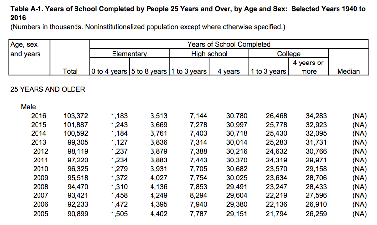
Data comes in an untidy form all the time, often for the good reason
that it can be presented that way using much less space, or with far
less repetition of labels and row elements. Figure
A.2 shows a the first few rows of a table of U.S.
Census Bureau data about educational attainment in the United States.
To begin with, it’s organized as a series of sub-tables down the
spreadsheet, broken out by age and sex. Second, the underlying
variable of interest, “Years of School Completed” is stored across
several columns, with an additional variable (level of schooling)
included across the columns also. It is not too hard to get the table
into a slightly more regular format by eliminating the blank rows, and
explicitly naming the sub-table rows. One can do this manually and get
to the point where it can be read in as an Excel or CSV file. This is
not ideal, as manually cleaning data runs against the commitment to do
as much as possible programmatically.readxl.tidyverse.org We can automate the process
somewhat. The tidyverse comes with a readxl package that tries to
ease the pain a little.
Figure A.2: Untidy data from the Census.
## # A tibble: 366 x 11
##    age   sex    year total elem4 elem8   hs3   hs4 coll3 coll4 median
##    <chr> <chr> <int> <int> <int> <int> <dbl> <dbl> <dbl> <dbl>  <dbl>
##  1 25-34 Male   2016 21845   116   468  1427  6386  6015  7432     NA
##  2 25-34 Male   2015 21427   166   488  1584  6198  5920  7071     NA
##  3 25-34 Male   2014 21217   151   512  1611  6323  5910  6710     NA
##  4 25-34 Male   2013 20816   161   582  1747  6058  5749  6519     NA
##  5 25-34 Male   2012 20464   161   579  1707  6127  5619  6270     NA
##  6 25-34 Male   2011 20985   190   657  1791  6444  5750  6151     NA
##  7 25-34 Male   2010 20689   186   641  1866  6458  5587  5951     NA
##  8 25-34 Male   2009 20440   184   695  1806  6495  5508  5752     NA
##  9 25-34 Male   2008 20210   172   714  1874  6356  5277  5816     NA
## 10 25-34 Male   2007 20024   246   757  1930  6361  5137  5593     NA
## # ... with 356 more rows
The tidyverse has several tools to help you get the rest of the way in
converting your data from an untidy to a tidy state. These can mostly
be found in the tidyr and dplyr libraries. The former provides
functions for converting, for example, wide-format data to long-format
data, as well as assisting with the business of splitting and
combining variables that are untidily stored. The latter has a tools
that allow tidy tables to be further filtered, sliced, and analyzed at
different grouping levels, as we have seen throughout this book.
With our edu object, we can use the gather() function to transform
the schooling variables into a key-value arrangement. The key is the
underlying variable, and the value is the value it takes for that
observation. We create a new object, edu_t in this way.
edu_t <- gather(data = edu,
                key = school,
                value = freq,
                elem4:coll4)

head(edu_t)
## # A tibble: 6 x 7
## age sex year total median school freq
## <chr> <chr> <int> <int> <dbl> <chr> <dbl>
## 1 25-34 Male 2016 21845 NA elem4 116
## 2 25-34 Male 2015 21427 NA elem4 166
## 3 25-34 Male 2014 21217 NA elem4 151
## 4 25-34 Male 2013 20816 NA elem4 161
## 5 25-34 Male 2012 20464 NA elem4 161
## 6 25-34 Male 2011 20985 NA elem4 190tail(edu_t) ## # A tibble: 6 x 7
## age sex year total median school freq
## <chr> <chr> <int> <int> <dbl> <chr> <dbl>
## 1 55> Female 1959 16263 8.30 coll4 688
## 2 55> Female 1957 15581 8.20 coll4 630
## 3 55> Female 1952 13662 7.90 coll4 628
## 4 55> Female 1950 13150 8.40 coll4 436
## 5 55> Female 1947 11810 7.60 coll4 343
## 6 55> Female 1940 9777 8.30 coll4 219The educational categories previously spread over the columns have
been gathered into two new columns. The school variable is the key
column. It contains all of the education categories that were
previously given across the column headers, from 0-4 years of
elementary school to four or more years of college. They are now
stacked up on top of each other in the rows. The freq variable is
the value column, and contains the unique value of schooling for
each level of that variable. Once our data is in this long-form shape,
it is ready for easy use with ggplot and related tidyverse tools.
A.2 Common problems reading in data
Date formats
Date formats can be annoying. First, times and dates must be treated differently from ordinary numbers. Second, there are many, many different date formats, differing both in the precision with which they are stored and the convention they follow about how to display years, months, days, and so on. Consider the following data:
head(bad_date)## # A tibble: 6 x 2
## date N
## <chr> <int>
## 1 9/1/11 44426
## 2 9/2/11 55112
## 3 9/3/11 19263
## 4 9/4/11 12330
## 5 9/5/11 8534
## 6 9/6/11 59490The data in the date column has been read in as a character
string, but we want R to treat it as a date. If can’t treat it as a
date, we get bad results.
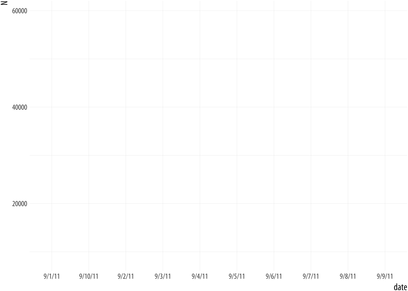 Figure A.3: A bad date.
p <- ggplot(data = bad_date, aes(x = date, y = N))
p + geom_line()
## geom_path: Each group consists of only one observation.
## Do you need to adjust the group aesthetic?What has happened? The problem is that ggplot doesn’t know date
consists of dates. As a result, when we ask to plot it on the x-axis,
it tries to treat the unique elements of date like a categorical
variable instead. (That is, as a factor.) But because each date is
unique, its default effort at grouping the data results in every group
having only one observation in it (i.e., that particular row). The
ggplot function knows something is odd about this, and tries to let
you know. It wonders whether we’ve failed to set group = <something>
in our mapping.
For the sake of it, let’s see what happens when the bad date values
are not unique. We will make a new data frame by stacking two copies of
the data on top of each other. The rbind() function does this for
us. We end up with two copies of every observation.
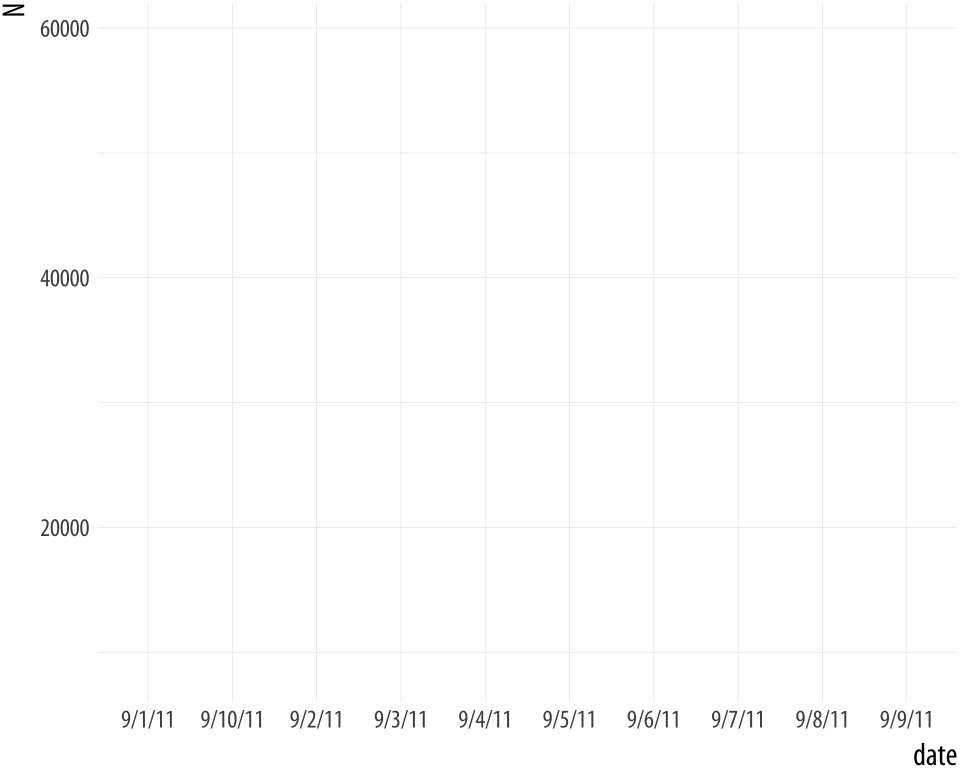 Figure A.4: Still bad.
bad_date2 <- rbind(bad_date, bad_date)

p <- ggplot(data = bad_date2, aes(x = date, y = N))
p + geom_line()
Now ggplot doesn’t complain at all, because there’s more than one observation per (inferred) group. But the plot is still wrong!
We will fix this problem using the lubridate library. It provides a
suite of convenience functions for converting date strings in various
formats and with various separators (such as / or - and so on)
into objects of class Date that R knows about. Here our bad dates
are in a month/day/year format, so we use mdy(). Consult the
lubridate library’s documentation to learn more about similar
convenience functions for converting character strings where the date
components appear in a different order.
# install.packages("lubridate")
library(lubridate)

bad_date$date <- mdy(bad_date$date)
head(bad_date)
## # A tibble: 6 x 2
## date N
## <date> <int>
## 1 2011-09-01 44426
## 2 2011-09-02 55112
## 3 2011-09-03 19263
## 4 2011-09-04 12330
## 5 2011-09-05 8534
## 6 2011-09-06 59490Now filldate_new has a Date class. Let’s try the plot
again.
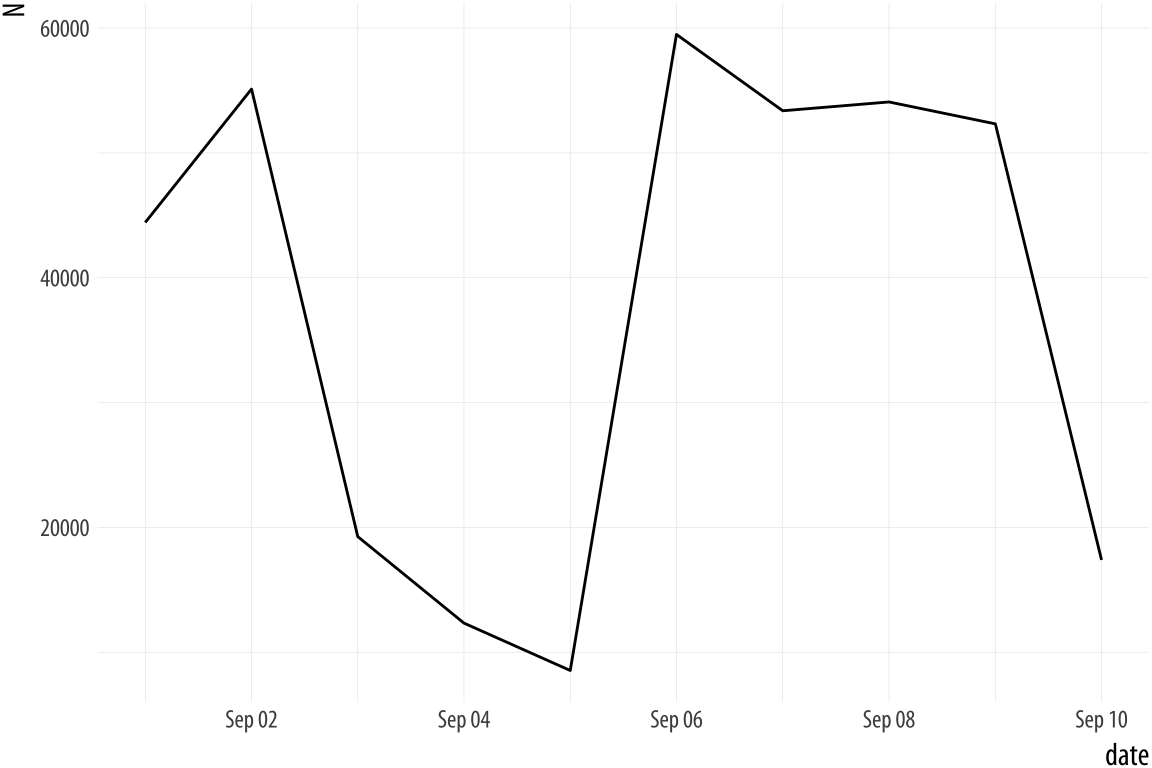 Figure A.5: Much better.
p <- ggplot(data = bad_date, aes(x = date, y = N))
p + geom_line()
Year-only dates
Many variables are measured by the year and supplied in the data as a four digit number rather than as a date. This can sometimes cause headaches when we want to plot year on the x-axis. It happens most often when the time series is relatively short. Consider this data:
url <- "https://cdn.rawgit.com/kjhealy/viz-organdata/master/organdonation.csv"

bad_year <- read_csv(url)
bad_year %>% select(1:3) %>% sample_n(10)
## # A tibble: 10 x 3
## country year donors
## <chr> <int> <dbl>
## 1 United States 1994 19.4
## 2 Australia 1999 8.67
## 3 Canada 2001 13.5
## 4 Australia 1994 10.2
## 5 Sweden 1993 15.2
## 6 Ireland 1992 19.5
## 7 Switzerland 1997 14.3
## 8 Ireland 2000 17.6
## 9 Switzerland 1998 15.4
## 10 Norway NA NAThis is a version of organdata but in a less clean format. The year variable is an integer (its class is <int>) and not a date. Let’s say we want to plot donation rate against year.
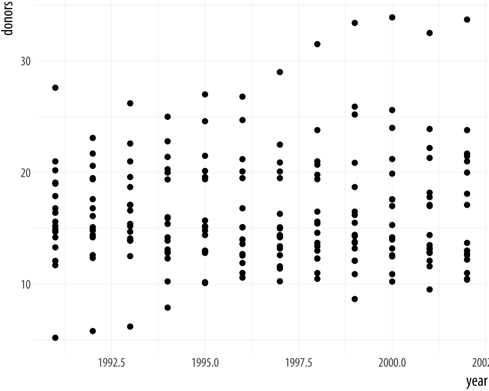 Figure A.6: Integer year shown with a decimal point.
p <- ggplot(data = bad_year, aes(x = year, y = donors))
p + geom_point()
The decimal point on the x-axis labels is unwanted. We could sort this out cosmetically, by giving scale_x_continuous() a set of breaks and labels that represent the years as characters. Alternatively, we can change the class of the year variable. For convenience, we will tell R that the year variable should be treated as a Date measure, and not an integer. We’ll use a home-cooked function, int_to_year(), that takes
integers and converts them to dates.
bad_year$year <- int_to_year(bad_year$year)
bad_year %>% select(1:3)
## # A tibble: 238 x 3
## country year donors
## <chr> <date> <dbl>
## 1 Australia NA NA
## 2 Australia 1991-01-01 12.1
## 3 Australia 1992-01-01 12.4
## 4 Australia 1993-01-01 12.5
## 5 Australia 1994-01-01 10.2
## 6 Australia 1995-01-01 10.2
## 7 Australia 1996-01-01 10.6
## 8 Australia 1997-01-01 10.3
## 9 Australia 1998-01-01 10.5
## 10 Australia 1999-01-01 8.67
## # ... with 228 more rowsIn the process, today’s day and month are introduced into the year data, but that is irrelevant in this case, given that our data are only observed in a yearly window to begin with. However, if you wish to specify a generic day and month for all the observations, the function allows you to do this.
A.2.1 Write functions for repetitive tasks
If you are working with a data set that you will be making a lot of similar plots from, or will need to periodically look at in a way that is repetitive but can’t be carried out in a single step once and for all, then the chances are that you will start accumulating sequences of code that you find yourself using repeatedly. When this happens, the temptation will be to start copying and pasting these sequences from one analysis to the next. We can see something of this tendency in the code samples for this book. To make the exposition clearer, we have periodically repeated chunks of code that differ only in the dependent or independent variable being plotted.
You should try to avoid copying and pasting code repeatedly in this way. Instead, this is an opportunity to write a function to help you out a little. More or less everything in R is accomplished through functions, and it’s not too difficult to write your own. This is especially the case when you begin by thinking of functions as a way to help you automate some local or smaller task, rather than a means of accomplishing some very complex task. R has the resources to help you build complex functions and function libraries, like ggplot itself. But we can start quite small, with functions that help us manage a particular dataset or data analysis.
Remember, functions take inputs, perform actions, and return outputs. For example, imagine a function that adds two numbers, x and y. In use, it might look like this:
add_xy(x = 1, y = 7)## [1] 8How do we create this function? Remember, everything is an object, so functions are just special kinds of object. And everything in R is done via functions. So, if we want to make a new function we will use an existing function do to it. In R, functions are created with function():
add_xy <- function(x, y) {
    x + y
}
You can see that function() is a little different from ordinary functions in two ways. First, the arguments we give it (here, x and y) are for the add_xy function that we are creating. Second, immediately after the function(x, y) statement there’s an opening brace, {, followed by a bit of R code that adds x and y, and then the closing brace }. That’s the content of the function. We assign this code to the add_xy object, and now we have a function that adds two numbers together and returns the result. The x + y line inside the parentheses is evaluated as if it were typed at the console, assuming you have told it what x and y are.
add_xy(x = 5, y = 2)## [1] 7Functions can take many kinds of arguments, and we can also tell them
what the default value of each argument should be by specifying it
inside the function(...) section. Functions are little programs that
have all the power of R at their disposal, including standard things
like flow-control through if ... else statements and so on. Here,
for instance, is a function that will make a scatter plot for any
Section in the ASA data, or optionally fit a smoother to the data
and plot that instead. Defining a function looks a little like calling one, except that we spell out the steps inside. We also specify the default arguments.
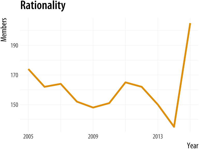
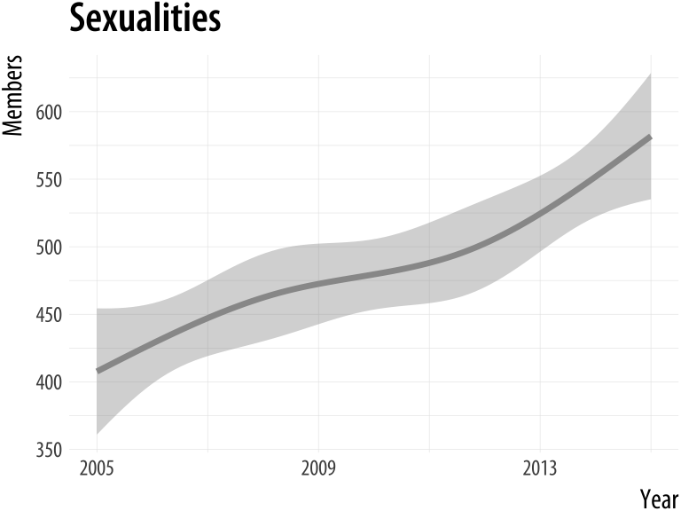
plot_section <- function(section="Culture", x = "Year",
                         y = "Members", data = asasec,
                         smooth=FALSE){
    require(ggplot2)
    require(splines)
    # Note use of aes_string() rather than aes()
    p <- ggplot(subset(data, Sname==section),
            mapping = aes_string(x=x, y=y))

    if(smooth == TRUE) {
        p0 <- p + geom_smooth(color = "#999999",
                              size = 1.2, method = "lm",
                              formula = y ~ ns(x, 3)) +
            scale_x_continuous(breaks = c(seq(2005, 2015, 4))) +
            labs(title = section)
    } else {
    p0 <- p + geom_line(color= "#E69F00", size=1.2) +
        scale_x_continuous(breaks = c(seq(2005, 2015, 4))) +
        labs(title = section)
    }

    print(p0)
}
This function is not very general. Nor is it particularly robust. But for the use we want to put it to, it works just fine.
plot_section("Rationality")
plot_section("Sexualities", smooth = TRUE)
Figure A.7: Using a function to plot your results.
If we were going to work with this data for long enough, we could make
the function progressively more general. For example, we can add the
special ... argument (which means, roughly, “and any other named
arguments”) in a way that allows us to pass arguments through to the
geom_smooth() function in the way we’d expect if we were using it
directly. With that in place, we can pick the smoothing method we want.
plot_section <- function(section="Culture", x = "Year",
                         y = "Members", data = asasec,
                         smooth=FALSE, ...){
    require(ggplot2)
    require(splines)
    # Note use of aes_string() rather than aes()
    p <- ggplot(subset(data, Sname==section),
            mapping = aes_string(x=x, y=y))

    if(smooth == TRUE) {
        p0 <- p + geom_smooth(color = "#999999",
                              size = 1.2, ...) +
            scale_x_continuous(breaks = c(seq(2005, 2015, 4))) +
            labs(title = section)
    } else {
    p0 <- p + geom_line(color= "#E69F00", size=1.2) +
        scale_x_continuous(breaks = c(seq(2005, 2015, 4))) +
        labs(title = section)
    }

    print(p0)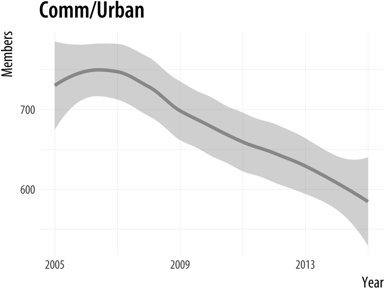
}plot_section("Comm/Urban",
smooth = TRUE,
method = "loess")
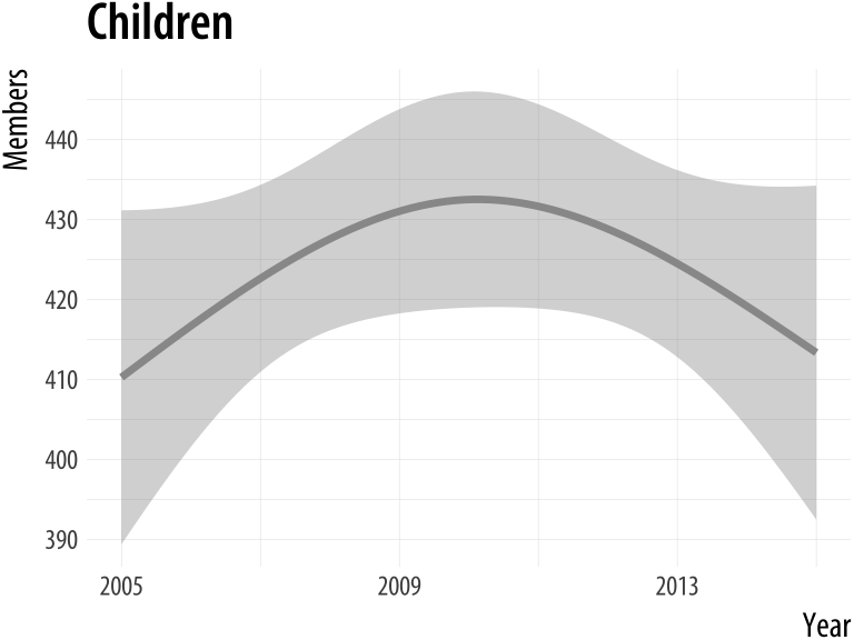
plot_section("Children",
smooth = TRUE,
method = "lm",
formula = y ~ ns(x, 2))Figure A.8: Our custom function can now pass arguments along to fit different smoothers to Section membership data.
A.3 Managing projects and files
A.3.1 RMarkdown and knitr
Markdownen.wikipedia.org/wiki/Markdown is a
loosely-standardized way of writing plain text that includes
information about the formatting of your document. It was originally
developed by John Gruber, with input from Aaron Swartz. The aim was to
make a simple format that could incorporate some structural
information about the document (such as headings and subheadings,
emphasis, hyperlinks, lists, footnotes, and so on), with minimal loss of readability in plain-text
form. A plain-text format like HTML is much more extensive and
well-defined than Markdown, but Markdown was meant to be simple. Over
the years, and despite various weaknesses, it has become a de facto
standard. Text editors and note-taking applications support it, and
tools exist to convert Markdown not just into HTML (its original
target output format) but many other document types as well. The most
powerful of these is Pandocpandoc.org, which can get you
from markdown to many other formats (and vice versa). Pandoc is what
powers RStudio’s ability to convert your notes to HTML, Microsoft
Word, and PDF documents.
Chapter 1 of this book encourages you to take notes and organize your
analysis using RMarkdownrmarkdown.rstudio.com and (behind the scenes) knitryihui.name/knitr. These are R libraries that RStudio makes easy to use. RMarkdown extends Markdown by letting
you intersperse your notes with chunks of R code. Code chunks can have
labels and a few options that determine how they will behave when the
file is processed. After writing your notes and your code, you knit
the document (Xie, 2015). That is, you feed your .Rmd file
to R, which processes the code chunks, and produces a new .md where
the code chunks have been replaced by their output. You can then turn
that Markdown file into a more readable PDF or HTML document, or the
Word document that a journal demands you send them.
Behind the scenes in RStudio, this is all done using the knitr and
rmarkdown libraries. The latter provides a render() function that
takes you from .Rmd to HTML or PDF in a single step. Conversely, if
you just want to extract the code you’ve written from the surrounding
text, then you “tangle” the file, which results in an .R file. The
strength of this approach is that is makes it much easier to document
your work properly. There is just one file for both the data analysis
and the writeup. The output of the analysis is created on the fly, and
the code to do it is embedded in the paper. If you need to do multiple
but identical (or very similar) analyses of different bits of data,
RMarkdown and knitr can make generating consistent and reliable
reports much easier.
Pandoc’s flavor of Markdown is the one used in knitr and RStudio. It allows for a wide range of markup, and can handle many of the nuts and bolts of scholarly writing, such as complex tables, citations, bibliographies, references, and mathematics. In addition to being able to produce documents in various file formats, it can also produce many different kinds of document, from articles and handouts to websites and slide decks. RStudio’s RMarkdown website has extensive documentation and examples on the ins and outs of RMarkdown’s capabilities, including information on customizing it if you wish.
Writing your notes and papers in a plain text format like this has many advantages. It keeps your writing, your code, and your results closer together, and allows you to use powerful version control methods to keep track of your work and your results. Errors in data analysis often well up out of the gap that typically exists between the procedure used to produce a figure or table in a paper and the subsequent use of that output later. In the ordinary way of doing things, you have the code for your data analysis in one file, the output it produced in another, and the text of your paper in a third file. You do the analysis, collect the output and copy the relevant results into your paper, often manually reformatting them on the way. Each of these transitions introduces the opportunity for error. In particular, it is easy for a table of results to get detached from the sequence of steps that produced it. Almost everyone who has written a quantitative paper has been confronted with the problem of reading an old draft containing results or figures that need to be revisited or reproduced (as a result of peer-review, say) but which lack any information about the circumstances of their creation. Academic papers take a long time to get through the cycle of writing, review, revision, and publication, even when you’re working hard the whole time. It is not uncommon to have to return to something you did two years previously in order to answer some question or other from a reviewer. You do not want to have to do everything over from scratch in order to get the right answer. I am not exaggerating when I say that, whatever the challenges of replicating the results of someone else’s quantitative analysis, after a fairly short period of time authors themselves find it hard to replicate their own work. Bit-rot is the term of art in Computer Science for the seemingly inevitable process of decay that overtakes a project just because you left it alone on your computer for six months or more.
For small and medium-sized projects, plain text approaches that rely on RMarkdown documents and the tools described here work well. Things become a little more complicated as projects get larger. (This is not an intrinsic flaw of plain-text methods, by the way. It is true no matter how you choose to organize your project.) In general, it is worth trying to keep your notes and analysis in a standardized and simple format. The final outputs of projects (such as journal articles or books) tend, as they approach completion, to descend into a rush of specific fixes and adjustments, all running against the ideal of a fully portable, reproducible analysis. It is worth trying to minimize the scope of the inevitable final scramble.
A.3.2 Project organization
Managing projects is a large topic of its own, and one that people have strong opinions about. Your goal should be to make your code and data portable, reproducible, and self-contained. In practice that means using a project based approach in R Studio. When you start an analysis with some new data, create a new project containing the data and the R or RMarkdown code you will be working with. It should then be possible, in the ideal case, to move that folder to another computer that also has R, RStudio, and any required libraries installed, and successfully re-run the contents of the project.
In practice that means two things. First, even though R is an object-oriented language, the only “real”, persistent things in your project should be the raw data files you start with, and the code that operates on them. The code is what is real. Your code manipulates the data and creates all of the objects and outputs you need. It’s possible to save objects in R but in general you should not need to do this for everyday analysis.
Second, your code should not refer to any file locations outside of the project folder. The project folder should be the “root” or ground floor for the files inside it. This means you should not use absolute file paths to save or refer to data or figures. Instead, use only relative paths. A relative path will start at the root of the project. So, for example, you should not load data with a command like this:
## An absolute file path.
## Notice the leading "/" that starts at the very top
## of the computer's file hierarchy.
my_data <- read_csv("/Users/kjhealy/projects/gss/data/gss.csv")
Instead, because you have an R project file started in the gss folder you can use the here() library to specify a relative path, like this:
my_data <- read_csv(here("data", "gss.csv"))While you could type the relative paths out yourself, using here() has the advantage that it will work if, for example, you use Mac OS and you send your project to someone working on Windows. The same rule goes for saving your work, as we saw at the end of Chapter @(sec:makeplot), when you save individual plots as PDF or PNG files.
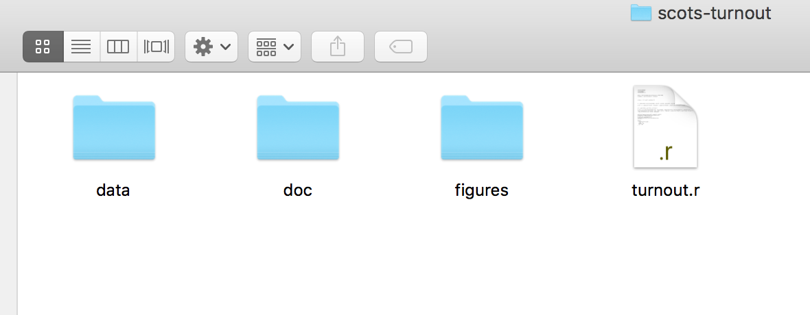 Figure A.9: Folder organization for a simple project.
Within your project folder, a little organization goes a long way. You should get in the habit of keeping different parts of the project in different sub-folders of your working directory. More complex projects may have a more complex structure, but you can go a long way with some simple organization. RMarkdown files can be in the top level of your working directory, with separate sub-folders called data/ (for your CSV files), one for figures/ (that you might save) and perhaps one called docs/ for information about your project or data files files. Rstudio can help with organization as well through its project management features.
Keeping your project organized just a little bit will prevent you from ending up with huge numbers of files of different kinds all sitting at the top of your working directory.
A.4 Some features of this book
A.4.1 Preparing the county-level maps
The U.S. county-level maps in the socviz library were prepared using
shapefiles from the U.S. Census Bureau that were converted to GeoJSON
format by Eric Celeste.eric.clst.org/Stuff/USGeoJSON The code to prepare the imported shapefile was written by Bob Rudis, and draws on the rgdal library to do the heavy lifting of importing the shapefile and transforming the projection. Bob’s code extracts the (county-identifying) rownames from the imported spatial data frame, and then moves Alaska and Hawaii to new locations in the bottom left of the map area, so that we can map all fifty states instead of just the lower forty eight.
First we read in the map file, set the projection, and set up an identifying variable we can work with later on to merge in data. The call to CRS() is a single long line of text conforming to a technical GIS specification defining the projection and other details that the map is encoded in. Long lines of code are conventionally indicated by the backslash charater, “\”, when we have to artificially break them on the page. Do not type the backslash if you write out this code yourself. We assume the mapfile is named gz_2010_us_050_00_5m.json and is in the data/geojson subfolder of the project directory.
# You will need to use install.packages() to install
# these map and GIS libraries if you do not already
# have them.

library(maptools)
library(mapproj)
library(rgeos)
library(rgdal)

us_counties <- readOGR(dsn="data/geojson/gz_2010_us_050_00_5m.json",
                       layer="OGRGeoJSON")

us_counties_aea <- spTransform(us_counties,
                    CRS("+proj=laea +lat_0=45 +lon_0=-100 \
                         +x_0=0 +y_0=0 +a=6370997 +b=6370997 \
                         +units=m +no_defs"))

us_counties_aea@data$id <- rownames(us_counties_aea@data)
With the file imported, we then extract, rotate, shrink, and move Alaska, resetting the projection in the process. We also move Hawaii. The areas are identified by their State FIPS codes. We remove the old states and put the new ones back in, and remove Puerto Rico as our examples lack data for this region. If you have data for the area, you can move it between Texas and Florida.
alaska <- us_counties_aea[us_counties_aea$STATE == "02",]
alaska <- elide(alaska, rotate=-50)
alaska <- elide(alaska, scale=max(apply(bbox(alaska), 1, diff)) / 2.3)
alaska <- elide(alaska, shift=c(-2100000, -2500000))
proj4string(alaska) <- proj4string(us_counties_aea)

hawaii <- us_counties_aea[us_counties_aea$STATE=="15",]
hawaii <- elide(hawaii, rotate=-35)
hawaii <- elide(hawaii, shift=c(5400000, -1400000))
proj4string(hawaii) <- proj4string(us_counties_aea)

us_counties_aea <- us_counties_aea[!us_counties_aea$STATE %in% c("02", "15", "72"),]
us_counties_aea <- rbind(us_counties_aea, alaska, hawaii)
Finally, we tidy the spatial object into a data frame that ggplot can use, and clean up the id label by stripping out a prefix from the string.
county_map <- tidy(us_counties_aea, region = "GEO_ID")
county_map$id <- stringr::str_replace(county_map$id,
pattern = "0500000US", replacement = "")AtFor more detail and code for the merge, see github.com/kjhealy/us-county this point the county_map object is ready to be merged with a table of FIPS-coded US county data using either merge() or left_join().
A.4.2 This book’s plot theme, and its map theme
The ggplot theme used in this book is derived principally from the work (again) of
Bob Rudis. His hrbrthemes package provides theme_ipsum(), a compact theme that can be used with the Arial typeface or, in a variant, the freely available Roboto Condensed typeface. The main difference between the theme_book() used here and Rudis’s theme_ipsum() is the choice of typeface. The hrbrthemes package can be installed from GitHub in the usual way:
devtools::install_github("hrbrmstr/hrbrthemes")Thegithub.com/kjhealy/myriad book theme is also available on GitHub. This package does not include the font files themselves. These are available from Adobe, who make the typeface.
When drawing maps we also used a theme_map() function. This theme
begins with the built-in theme_bw() and turns off most of the
guide, scale, panel content that is not needed when presenting a map. It is available through the socviz library. The code looks like this:
theme_map <- function(base_size=9, base_family="") {
    require(grid)
    theme_bw(base_size=base_size, base_family=base_family) %+replace%
        theme(axis.line=element_blank(),
              axis.text=element_blank(),
              axis.ticks=element_blank(),
              axis.title=element_blank(),
              panel.background=element_blank(),
              panel.border=element_blank(),
              panel.grid=element_blank(),
              panel.spacing=unit(0, "lines"),
              plot.background=element_blank(),
              legend.justification = c(0,0),
              legend.position = c(0,0)
              )
}
Themes are functions. Creating a theme means writing a function with a sequence of instructions about what thematic elements to modify, and how. We give it a default base_size argument and an empty base_family argument (for the font family). The %+replace% operator in the code is new to us. This is a convenience operator defined by ggplot and used for updating theme elements in bulk. Throughout the book we saw repeated use of the + operator to incrementally add to or tweak the content of a theme, as when we would do + theme(legend.position = "top"). Using + added the instruction to the theme, adjusting whatever was specified and leaving everything else as it was. The %+replace% operator does something similar, but it has a stronger effect. We begin with theme_bw() and then use a theme() statement to add new content, as usual. The %+replace% operator replaces the entire element specified, rather than adding to it. Any element not specified in the theme() statement will be deleted from the new theme. So this is a way to create themes by both starting from existing ones, specifying new elements, and deleting anything not explicitly mentioned. See the documentation for theme_get() for more details. In the function here, you can see each of the thematic elements that are “switched off” using the element_blank() function.